The Pandas DataFrame – loading, editing, and viewing data in Python

Starting out with Python Pandas DataFrames

If you’re developing in data science, and moving from excel-based analysis to the world of Python, scripting, and automated analysis, you’ll come across the incredibly popular data management library, “Pandas” in Python. Pandas development started in 2008 with main developer Wes McKinney and the library has become a standard for data analysis and management using Python. Pandas fluency is essential for any Python-based data professional, people interested in trying a Kaggle challenge, or anyone seeking to automate a data process.

The aim of this post is to help beginners get to grips with the basic data format for Pandas – the DataFrame. We will examine basic methods for creating data frames, what a DataFrame actually is, renaming and deleting data frame columns and rows, and where to go next to further your skills.

The topics in this post will enable you (hopefully) to:

1. Load your data from a file into a Python Pandas DataFrame,
2. Examine the basic statistics of the data,
3. Change some values,
4. Finally output the result to a new file.

What is a Python Pandas DataFrame?

The Pandas library documentation defines a DataFrame as a “two-dimensional, size-mutable, potentially heterogeneous tabular data structure with labeled axes (rows and columns)”. In plain terms, think of a DataFrame as a table of data, i.e. a single set of formatted two-dimensional data, with the following characteristics:

• There can be multiple rows and columns in the data.
• Each row represents a sample of data,
• Each column contains a different variable that describes the samples (rows).
• The data in every column is usually the same type of data – e.g. numbers, strings, dates.
• Usually, unlike an excel data set, DataFrames avoid having missing values, and there are no gaps and empty values between rows or columns.

By way of example, the following data sets that would fit well in a Pandas DataFrame:

• In a school system DataFrame – each row could represent a single student in the school, and columns may represent the students name (string), age (number), date of birth (date), and address (string).
• In an economics DataFrame, each row may represent a single city or geographical area, and columns might include the the name of area (string), the population (number), the average age of the population (number), the number of households (number), the number of schools in each area (number) etc.
• In a shop or e-commerce system DataFrame, each row in a DataFrame may be used to represent a customer, where there are columns for the number of items purchased (number), the date of original registration (date), and the credit card number (string).

Creating Pandas DataFrames

We’ll examine two methods to create a DataFrame – manually, and from comma-separated value (CSV) files.

Manually entering data

The start of every data science project will include getting useful data into an analysis environment, in this case Python. There’s multiple ways to create DataFrames of data in Python, and the simplest way is through typing the data into Python manually, which obviously only works for tiny datasets.

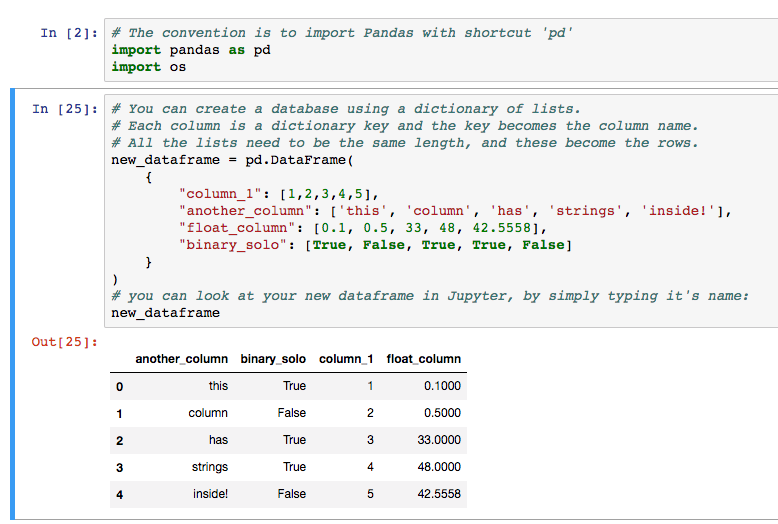
Note that convention is to load the Pandas library as ‘pd’ (import pandas as pd). You’ll see this notation used frequently online, and in Kaggle kernels.

Loading CSV data into Pandas

Creating DataFrames from CSV (comma-separated value) files is made extremely simple with the read_csv() function in Pandas, once you know the path to your file. A CSV file is a text file containing data in table form, where columns are separated using the ‘,’ comma character, and rows are on separate lines (see here).

If your data is in some other form, such as an SQL database, or an Excel (XLS / XLSX) file, you can look at the other functions to read from these sources into DataFrames, namely read_xlsx, read_sql. However, for simplicity, sometimes extracting data directly to CSV and using that is preferable.

In this example, we’re going to load Global Food production data from a CSV file downloaded from the Data Science competition website, Kaggle. You can download the CSV file from Kaggle, or directly from here. The data is nicely formatted, and you can open it in Excel at first to get a preview:

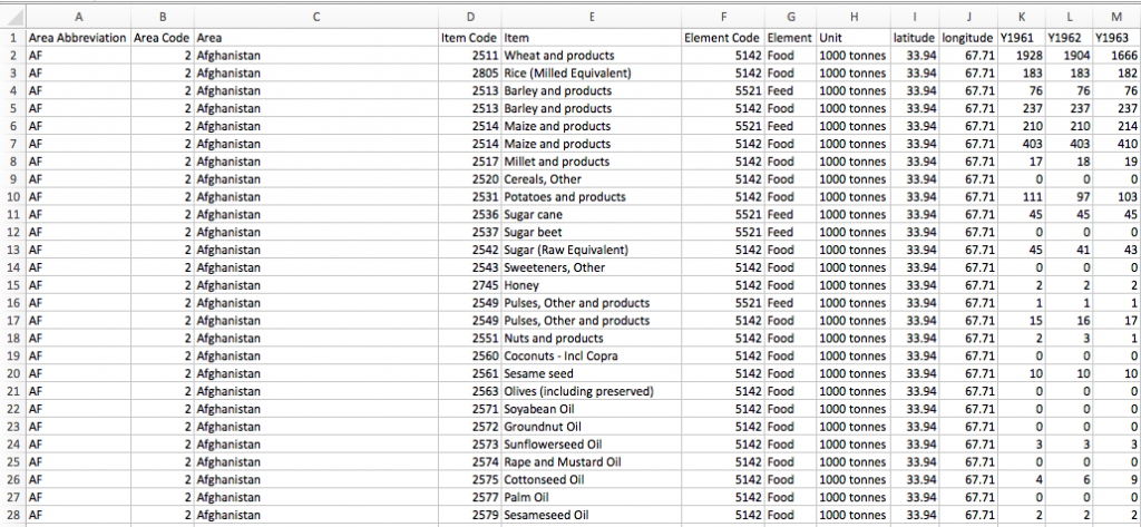
The sample data contains 21,478 rows of data, with each row corresponding to a food source from a specific country. The first 10 columns represent information on the sample country and food/feed type, and the remaining columns represent the food production for every year from 1963 – 2013 (63 columns in total).

If you haven’t already installed Python / Pandas, I’d recommend setting up Anaconda or WinPython (these are downloadable distributions or bundles that contain Python with the top libraries pre-installed) and using Jupyter notebooks (notebooks allow you to use Python in your browser easily) for this tutorial. Some installation instructions are here.

Load the file into your Python workbook using the Pandas read_csv function like so:

If you have path or filename issues, you’ll see FileNotFoundError exceptions like this:

FileNotFoundError: File b'https://c8j9w8r3.rocketcdn.me/some/directory/on/your/system/FAO+database.csv' does not exist

Preview and examine data in a Pandas DataFrame

Once you have data in Python, you’ll want to see the data has loaded, and confirm that the expected columns and rows are present.

Print the data

If you’re using a Jupyter notebook, outputs from simply typing in the name of the data frame will result in nicely formatted outputs. Printing is a convenient way to preview your loaded data, you can confirm that column names were imported correctly, that the data formats are as expected, and if there are missing values anywhere.

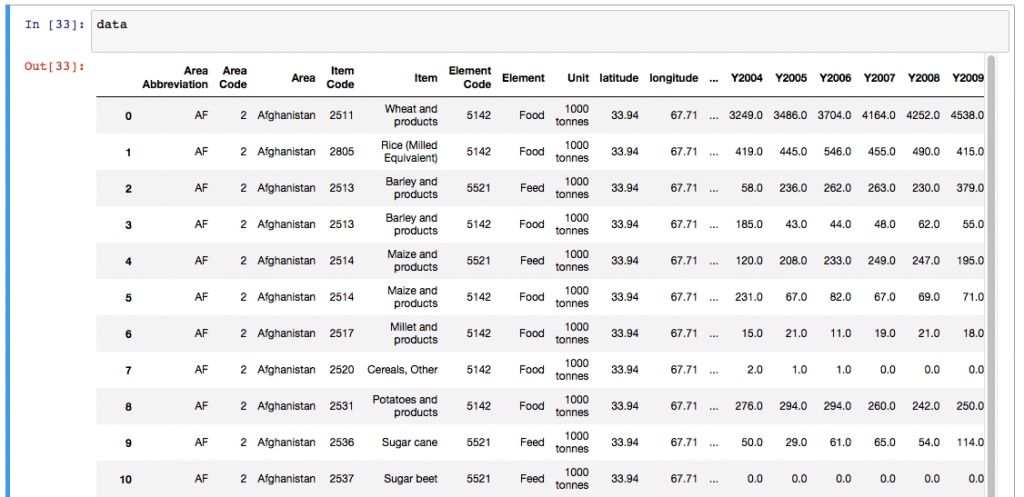
You’ll notice that Pandas displays only 20 columns by default for wide data dataframes, and only 60 or so rows, truncating the middle section. If you’d like to change these limits, you can edit the defaults using some internal options for Pandas displays (simple use pd.options.display.XX = value to set these):

• pd.options.display.width – the width of the display in characters – use this if your display is wrapping rows over more than one line.
• pd.options.display.max_rows – maximum number of rows displayed.
• pd.options.display.max_columns – maximum number of columns displayed.

You can see the full set of options available in the official Pandas options and settings documentation.

DataFrame rows and columns with .shape

The shape command gives information on the data set size – ‘shape’ returns a tuple with the number of rows, and the number of columns for the data in the DataFrame. Another descriptive property is the ‘ndim’ which gives the number of dimensions in your data, typically 2.

Our food production data contains 21,477 rows, each with 63 columns as seen by the output of .shape. We have two dimensions – i.e. a 2D data frame with height and width. If your data had only one column, ndim would return 1. Data sets with more than two dimensions in Pandas used to be called Panels, but these formats have been deprecated. The recommended approach for multi-dimensional (>2) data is to use the Xarray Python library.

Preview DataFrames with head() and tail()

The DataFrame.head() function in Pandas, by default, shows you the top 5 rows of data in the DataFrame. The opposite is DataFrame.tail(), which gives you the last 5 rows.

Pass in a number and Pandas will print out the specified number of rows as shown in the example below. Head() and Tail() need to be core parts of your go-to Python Pandas functions for investigating your datasets.

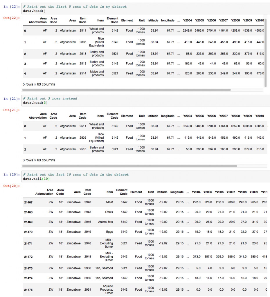
In our example here, you can see a subset of the columns in the data since there are more than 20 columns overall.

Data types (dtypes) of columns

Many DataFrames have mixed data types, that is, some columns are numbers, some are strings, and some are dates etc. Internally, CSV files do not contain information on what data types are contained in each column; all of the data is just characters. Pandas infers the data types when loading the data, e.g. if a column contains only numbers, pandas will set that column’s data type to numeric: integer or float.

You can check the types of each column in our example with the ‘.dtypes’ property of the dataframe.

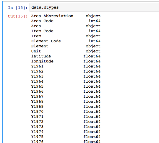
In some cases, the automated inferring of data types can give unexpected results. Note that strings are loaded as ‘object’ datatypes, because technically, the DataFrame holds a pointer to the string data elsewhere in memory. This behaviour is expected, and can be ignored.

To change the datatype of a specific column, use the .astype() function. For example, to see the ‘Item Code’ column as a string, use:

data['Item Code'].astype(str)

Describing data with .describe()

Finally, to see some of the core statistics about a particular column, you can use the ‘describe‘ function.

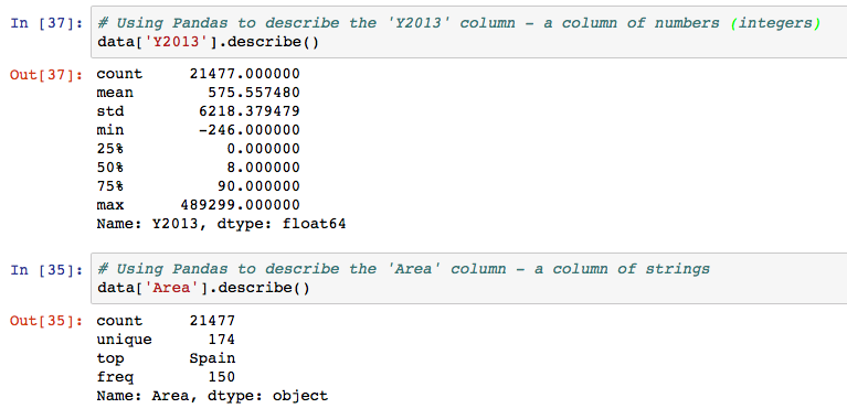
• For numeric columns, describe() returns basic statistics: the value count, mean, standard deviation, minimum, maximum, and 25th, 50th, and 75th quantiles for the data in a column.
• For string columns, describe() returns the value count, the number of unique entries, the most frequently occurring value (‘top’), and the number of times the top value occurs (‘freq’)

Select a column to describe using a string inside the [] braces, and call describe() as follows:

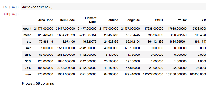
Note that if describe is called on the entire DataFrame, statistics only for the columns with numeric datatypes are returned, and in DataFrame format.

Selecting and Manipulating Data

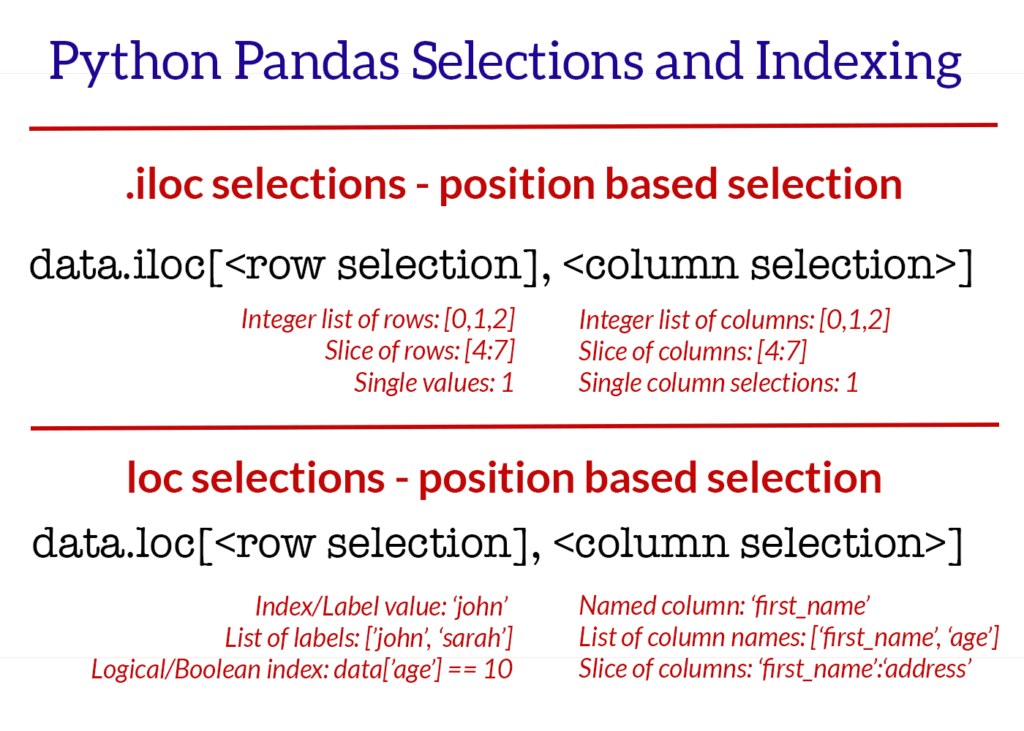
The data selection methods for Pandas are very flexible. In another post on this site, I’ve written extensively about the core selection methods in Pandas – namely iloc and loc. For detailed information and to master selection, be sure to read that post. For this example, we will look at the basic method for column and row selection.

Selecting columns

There are three main methods of selecting columns in pandas:

• using a dot notation, e.g. data.column_name,
• using square braces and the name of the column as a string, e.g. data['column_name']
• or using numeric indexing and the iloc selector data.iloc[:, <column_number>]

When a column is selected using any of these methodologies, a pandas.Series is the resulting datatype. A pandas series is a one-dimensional set of data. It’s useful to know the basic operations that can be carried out on these Series of data, including summing (.sum()), averaging (.mean()), counting (.count()), getting the median (.median()), and replacing missing values (.fillna(new_value)).

# Series summary operations.
# We are selecting the column "Y2007", and performing various calculations.
[data['Y2007'].sum(), # Total sum of the column values
 data['Y2007'].mean(), # Mean of the column values
 data['Y2007'].median(), # Median of the column values
 data['Y2007'].nunique(), # Number of unique entries
 data['Y2007'].max(), # Maximum of the column values
 data['Y2007'].min()] # Minimum of the column values

Out: [10867788.0, 508.48210358863986, 7.0, 1994, 402975.0, 0.0]

Selecting multiple columns at the same time extracts a new DataFrame from your existing DataFrame. For selection of multiple columns, the syntax is:

• square-brace selection with a list of column names, e.g. data[['column_name_1', 'column_name_2']]
• using numeric indexing with the iloc selector and a list of column numbers, e.g. data.iloc[:, [0,1,20,22]]

Selecting rows

Rows in a DataFrame are selected, typically, using the iloc/loc selection methods, or using logical selectors (selecting based on the value of another column or variable).

The basic methods to get your heads around are:

• numeric row selection using the iloc selector, e.g. data.iloc[0:10, :] – select the first 10 rows.
• label-based row selection using the loc selector (this is only applicably if you have set an “index” on your dataframe. e.g. data.loc[44, :]
• logical-based row selection using evaluated statements, e.g. data[data["Area"] == "Ireland"] – select the rows where Area value is ‘Ireland’.

Note that you can combine the selection methods for columns and rows in many ways to achieve the selection of your dreams. For details, please refer to the post “Using iloc, loc, and ix to select and index data“.

Deleting rows and columns (drop)

To delete rows and columns from DataFrames, Pandas uses the “drop” function.

To delete a column, or multiple columns, use the name of the column(s), and specify the “axis” as 1. Alternatively, as in the example below, the ‘columns’ parameter has been added in Pandas which cuts out the need for ‘axis’. The drop function returns a new DataFrame, with the columns removed. To actually edit the original DataFrame, the “inplace” parameter can be set to True, and there is no returned value.

# Deleting columns

# Delete the "Area" column from the dataframe
data = data.drop("Area", axis=1)

# alternatively, delete columns using the columns parameter of drop
data = data.drop(columns="area")

# Delete the Area column from the dataframe in place
# Note that the original 'data' object is changed when inplace=True
data.drop("Area", axis=1, inplace=True). 

# Delete multiple columns from the dataframe
data = data.drop(["Y2001", "Y2002", "Y2003"], axis=1)

Rows can also be removed using the “drop” function, by specifying axis=0. Drop() removes rows based on “labels”, rather than numeric indexing. To delete rows based on their numeric position / index, use iloc to reassign the dataframe values, as in the examples below.

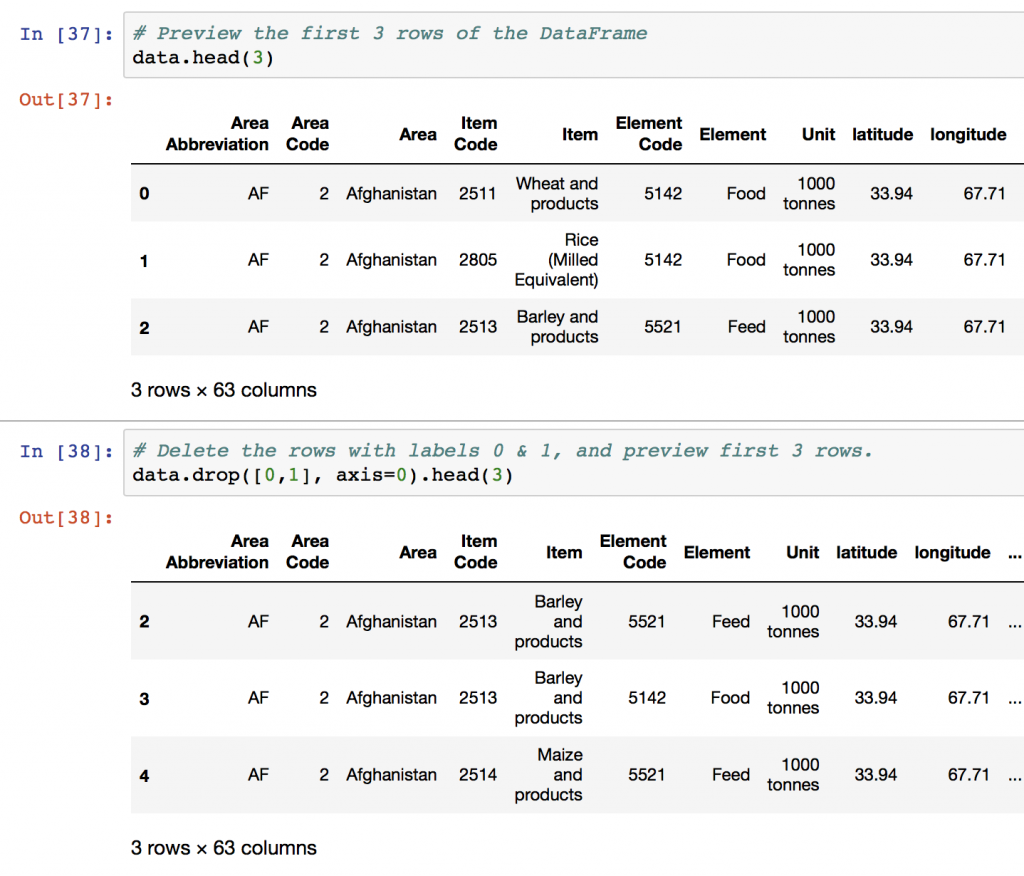
# Delete the rows with labels 0,1,5
data = data.drop([0,1,2], axis=0)

# Delete the rows with label "Ireland"
# For label-based deletion, set the index first on the dataframe:
data = data.set_index("Area")
data = data.drop("Ireland", axis=0). # Delete all rows with label "Ireland"

# Delete the first five rows using iloc selector
data = data.iloc[5:,]

Renaming columns

Column renames are achieved easily in Pandas using the DataFrame rename function. The rename function is easy to use, and quite flexible. Rename columns in these two ways:

• Rename by mapping old names to new names using a dictionary, with form {“old_column_name”: “new_column_name”, …}
• Rename by providing a function to change the column names with. Functions are applied to every column name.

# Rename columns using a dictionary to map values
# Rename the Area columnn to 'place_name'
data = data.rename(columns={"Area": "place_name"})

# Again, the inplace parameter will change the dataframe without assignment
data.rename(columns={"Area": "place_name"}, inplace=True)

# Rename multiple columns in one go with a larger dictionary
data.rename(
    columns={
        "Area": "place_name",
        "Y2001": "year_2001"
    },
    inplace=True
)

# Rename all columns using a function, e.g. convert all column names to lower case:
data.rename(columns=str.lower)

In many cases, I use a tidying function for column names to ensure a standard, camel-case format for variables names. When loading data from potentially unstructured data sets, it can be useful to remove spaces and lowercase all column names using a lambda (anonymous) function:

# Quickly lowercase and camelcase all column names in a DataFrame
data = pd.read_csv("https://c8j9w8r3.rocketcdn.me/path/to/csv/file.csv")
data.rename(columns=lambda x: x.lower().replace(' ', '_'))

Exporting and Saving Pandas DataFrames

After manipulation or calculations, saving your data back to CSV is the next step. Data output in Pandas is as simple as loading data.

Two two functions you’ll need to know are to_csv to write a DataFrame to a CSV file, and to_excel to write DataFrame information to a Microsoft Excel file.

# Output data to a CSV file
# Typically, I don't want row numbers in my output file, hence index=False.
# To avoid character issues, I typically use utf8 encoding for input/output.

data.to_csv("output_filename.csv", index=False, encoding='utf8')

# Output data to an Excel file.
# For the excel output to work, you may need to install the "xlsxwriter" package.

data.to_csv("output_excel_file.xlsx", sheet_name="Sheet 1", index=False)

Additional useful functions

Grouping and aggregation of data

As soon as you load data, you’ll want to group it by one value or another, and then run some calculations. There’s another post on this blog – Summarising, Aggregating, and Grouping Data in Python Pandas, that goes into extensive detail on this subject.

Plotting Pandas DataFrames – Bars and Lines

There’s a relatively extensive plotting functionality built into Pandas that can be used for exploratory charts – especially useful in the Jupyter notebook environment for data analysis.

You’ll need to have the matplotlib plotting package installed to generate graphics, and  the %matplotlib inline notebook ‘magic’ activated for inline plots. You will also need import matplotlib.pyplot as plt to add figure labels and axis labels to your diagrams. A huge amount of functionality is provided by the .plot() command natively by Pandas.

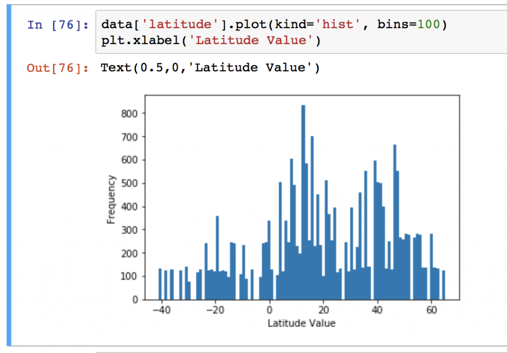
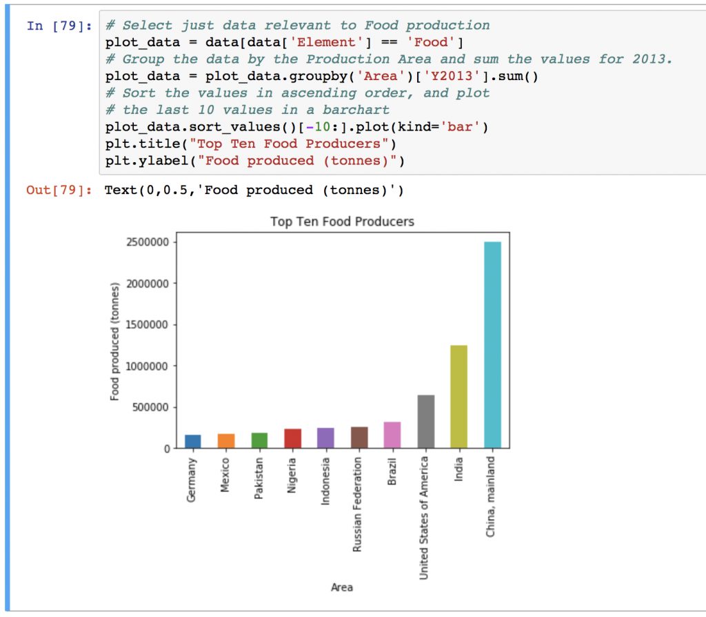
With enough interest, plotting and data visualisation with Pandas is the target of a future blog post – let me know in the comments below!

For more information on visualisation with Pandas, make sure you review:

• The official Pandas documentation on plotting and data visualisation.
• Simple Graphing with Python from Practical Business Python
• Quick and Dirty Data Analysis with Pandas from Machine Learning Mastery.

Going further

As your Pandas usage increases, so will your requirements for more advance concepts such as reshaping data and merging / joining (see accompanying blog post.). To get started, I’d recommend reading the 6-part “Modern Pandas” from Tom Augspurger as an excellent blog post that looks at some of the more advanced indexing and data manipulation methods that are possible.